*** This “how to” guide is now out of date – please use new guide (PDF) instead ***

Over recent weeks I have been working out ways to extract “top tweet” lists from huge extracts of Twitter data (NodeXL). A defining feature of Twitter is its immediacy. That presents challenges when attempting to summarise a large volume of activity – eg from an international conference (eg Quality2017 in London April 2017 – blog) or global public health campaign such as Immunization Week (read blog). Recent political events (eg science marches, UK’s June 2017 General Election) generated tens of thousands of tweets in hours or even minutes. I have attempted the step by step approach described below on a series of different extracts and it appears to work well.

NodeXL allows us to extract data on planned and unplanned social media activity, for a period of up to 9 days into the past. Sometimes a little bit of tweaking or patience is required to extract data.

NodeXL maps interactions around tweets, helping identify top tweeters, hashtags and quoted URLs. Sometimes, however, it is helpful to see the most dominant tweets; this identifies other content – eg popular infographics. Number of retweets is a measure of the popularity (or sometimes infamy) of a tweet, and I have used this measure to rank tweets (eg this for Antibiotic Awareness week, November 2016). For conferences I have then ranked the tweets chronologically (eg this for FISHIS16).

If you’re keen to try this out for yourself, here are a couple of large extracts to get your teeth into:

• An extract of last year’s American Public Health Association conference – see resulting Storify (top 179 tweets) here
• An extract of recent medical journal tweets (6 days to 30 June) – see resulting Storify (top 100 tweets) here

See my NodeXL extracts (and a few that mention ScotPublicHealth) here.

Have a go at following the step by step guide below, and let me know how you get on via Twitter.

*** I have updated (1 August 2017) to produce a simpler and quicker version (“New method” below), which I will compare with the original method ASAP. There are pros and cons of the two methods that I will describe when time ***

You’ll need Excel and a Storify account (free). If you have an Apple or Linux machine and want to produce your own step by step guide then please let me know and I’ll include on this page, giving you credit.

Graham Mackenzie (@gmacscotland on Twitter)

Consultant in Public Health

30 June 2017

New method

Follow steps 1-4 in original method below to download NodeXL file and “Edges” sheet.

For the example below I have used a search of tweets mentioning top medical journals or FOAMed (free open access medical education).

i) Select column N in “Edges” sheet and add two new columns

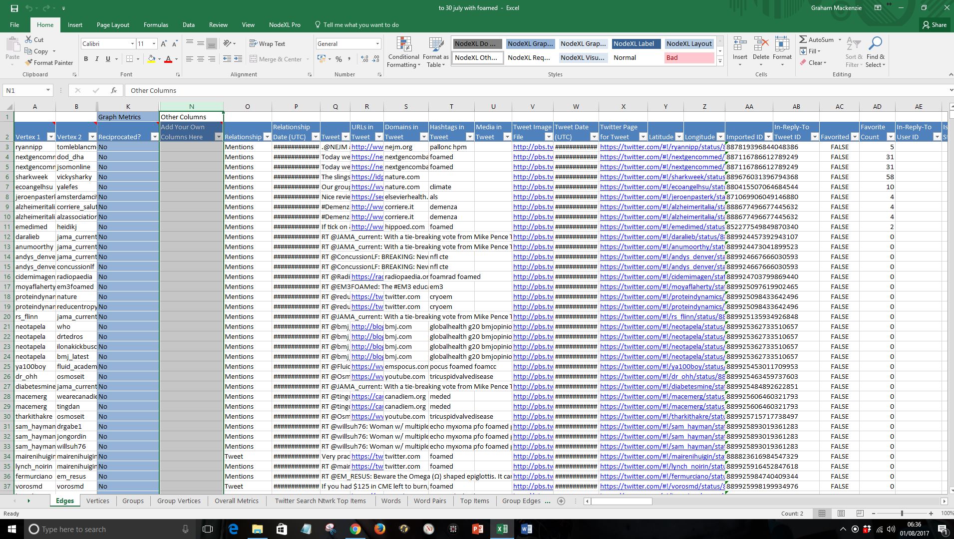
ii) Relabel these columns as “Original tweets (added)”, “Date (added)” and “URL (added)”.

iii) find original tweets by typing the following into cell N3

=IF(LEFT(S3,2)<>”RT”,S3,””)

Modern versions of Excel will copy this down to the bottom of the sheet. If this doesn’t happen automatically then do this yourself using copy and paste. 

iv) Find date if it is an original tweet by adding the following to cell O3

=IF(N3<>””,R3,””)

Again, copy and paste to bottom of sheet if this hasn’t happened automatically

Format this column to show date and time (custom format, dd/mm/yyyy hh:mm)

v) Find URL to tweet if it is an original tweet by adding the following to cell P3

=IF(N3<>””,Z3,””)

Again, copy and paste to bottom of sheet if this hasn’t happened automatically

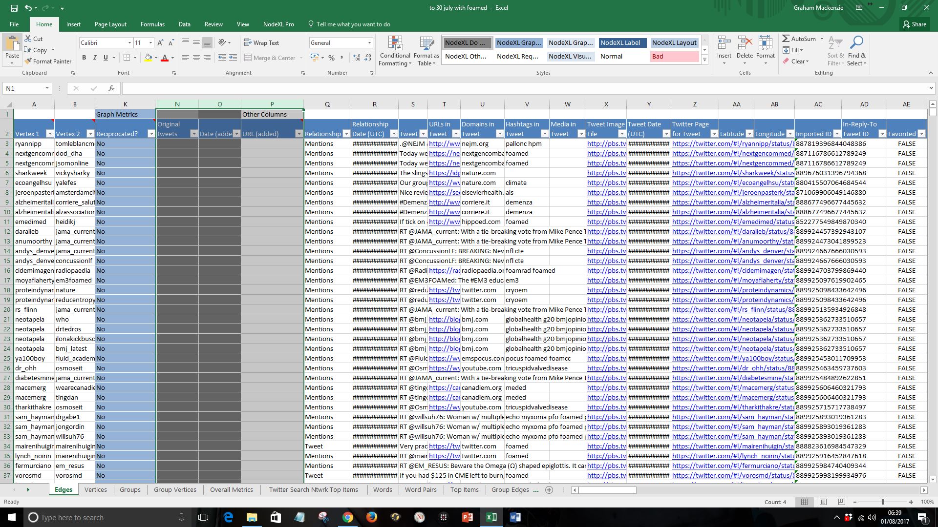
vi) Now insert another column (into column O) and table this as “RTs (added)”

Type in the following to find number of retweets if it is an original tweet by adding the following to cell O3

=IF(N3<>””,AN3,””)

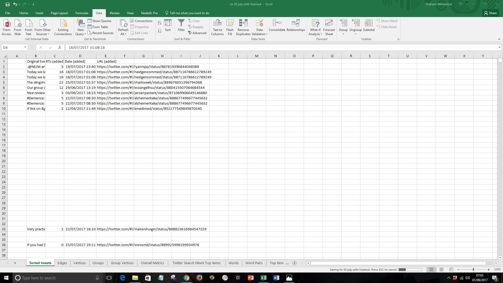
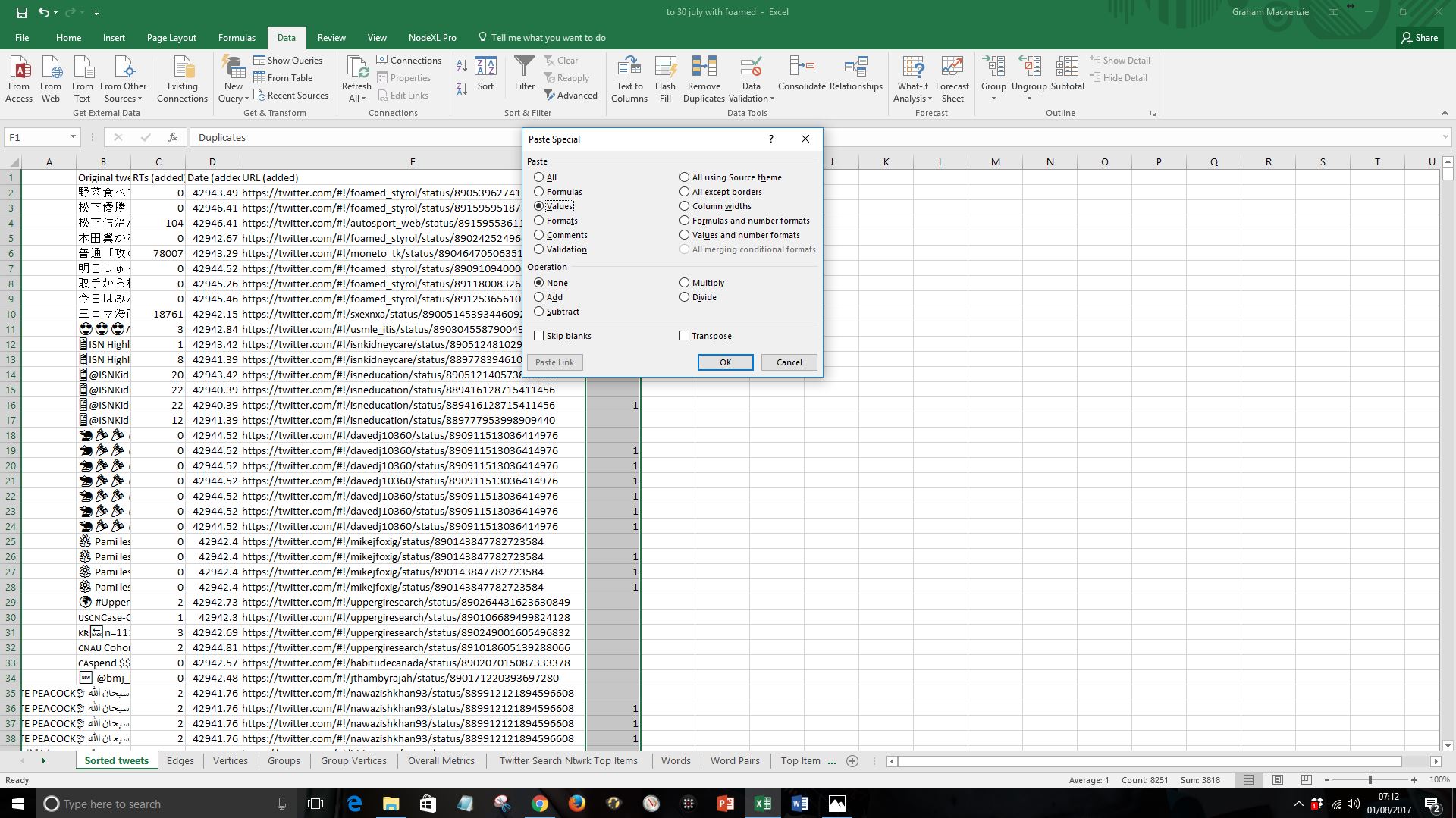
vii) Copy the 4 columns you have just generated and paste them into a new worksheet (paste special “values”, then format date column again to show date and time (custom format, dd/mm/yyyy hh:mm)

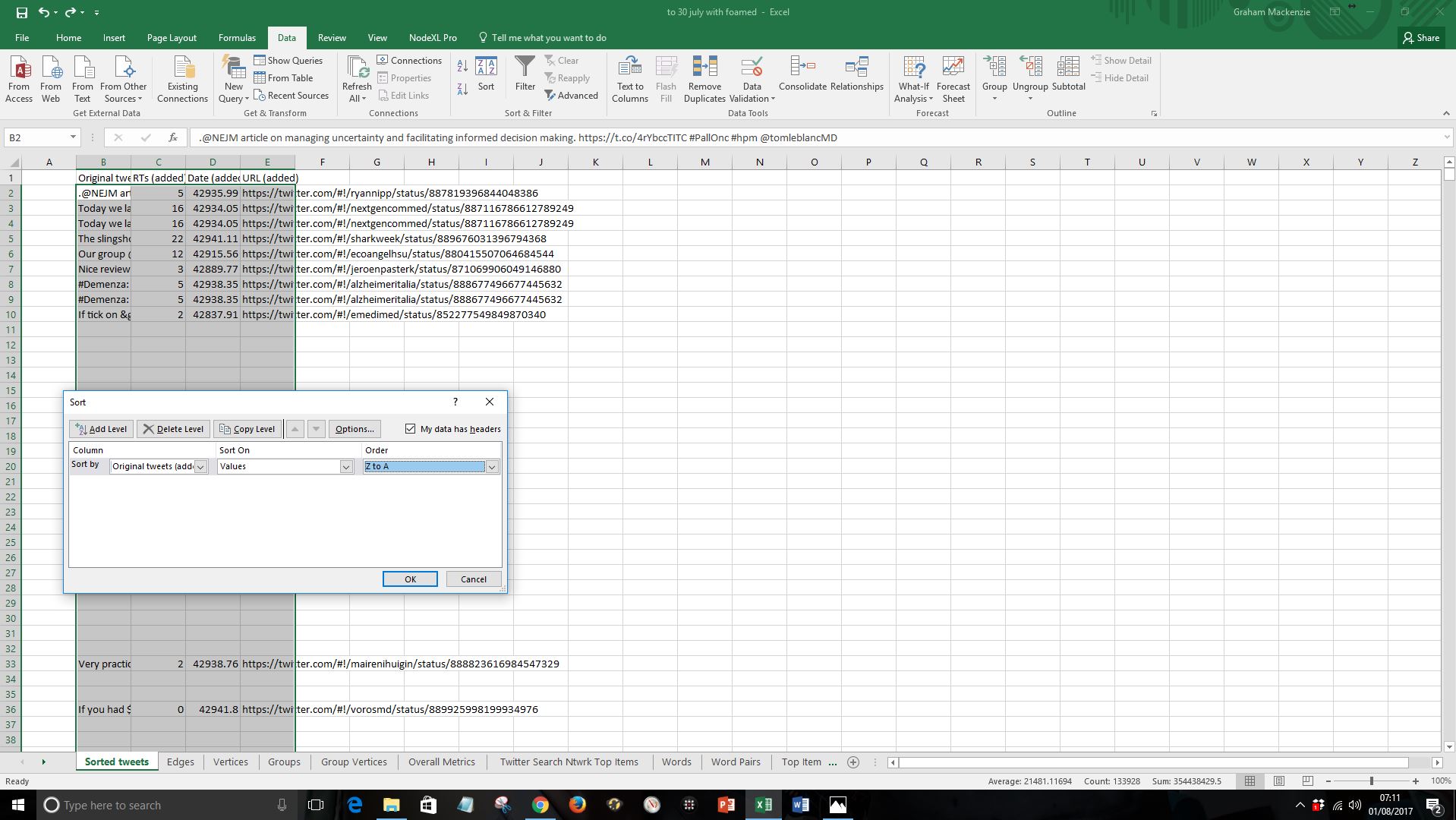
viii) Sort the four columns by “Original tweet” column (using Data: Sort). Here I have done this Z to A to avoid lots of blank rows. If you’d prefer to arrange it A to Z then delete the blank rows

NB – I spotted a flaw with the approach described in step viii when working on #WorldMentalHealthDay extract on 10 October 2017. If there are tweets with identical wording (as happens commonly for example when people post memes with just the hashtag in the body of the tweet) then it is better to sort by “URL” column. I will use this method from now onwards.

This step should therefore read: 

viii) Sort the four columns by “URL” column (using Data: Sort). 

ix) As you explore the tweets you’ll see a number of duplicates. Label column F as “Duplicates”

Type in the following into cell F2

=IF(E2=E1,1,””)

Copy this down to the bottom of the sheet. Then copy this column and “paste special: values”

Sort the five columns by the duplicates column, Z to A (using “Data: Sort”)

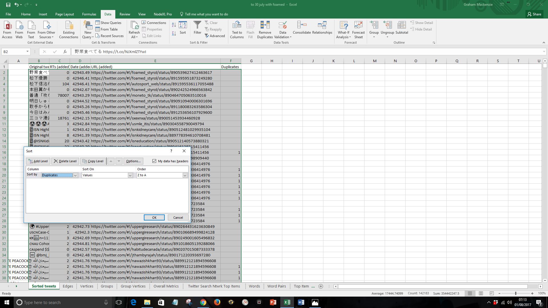
Delete the duplicate row (identified by “1” flag in the duplicate column)

x) Work out the period that you want to focus in on (date range). Produce a column (G) with dates, without times by typing in the following into cell G2

=DATE(YEAR(D2),MONTH(D2),DAY(D2))

Format column H as dates

Now type the start date of your selected period into cell H1

Type the following into cell H2, to identify tweets posted on or after that date and copy this down to the bottom of the sheet

=IF(G2>=H$1,1,””)

xi) Sort the sheet to show tweets posted during your selected period. Here I have ordered by number of retweets (descending) to show most popular tweets (first sorting by column H (largest to smallest), then by column C (largest to smallest).

Click on cell A2 and freeze panes (so that header shows when you scroll down to find your tweets). Scroll down to find tweets flagged with a “1” in column H.

Depending on your purpose you might want to add in further options. For example, for a conference you may want to focus in on tweets achieving a certain number of retweets, and arrange these chronologically. Read the text of the tweets in column B so that you can edit out irrelevant or unhelpful tweets, and copy and paste URL (from column E) into Storify summary as described in steps 29 onwards below.

 

or original method

Instructions	Image (click to view full size)
Step 1. Open up your chosen extract using NodeXL Graph Gallery website. Click here for NHSScotland17 extract for this worked example.
Step 2. Scroll down to link at bottom of page – “Download the Graph Data as a NodeXL Workbook” and download the related file
Step 3. Find the file (may be in your “downloads” folder) and move to a location of your choice. Open it up
Step 4. Select the “Edges” worksheet at the far left of the workbook
Step 5. Select the “Tweet” column (click on column “Q”)
Step 6. Copy and paste this column into a new workbook
Step 7. Click on “Tweet” at the top of this column and “select all” (hold down “control” key and press “A” key on a Windows PC). Insert a pivot table. This should open up in another worksheet
Step 8. In the pivot table fields box drop “Tweet” field into “Rows” and “Values”
Step 9. Select and copy all but the bottom row of the resulting pivot table (Select “Row labels” cell; hold down “control” key, press “A” key; release both keys; now hold down “shift key” and press “up” arrow; release; hold down “control” key again and press “C”)
Step 10. Paste the information alongside pivot table (click into a cell a couple of columns to right of pivot table, and paste the contents of the pivot table as “paste special”/ values). This gets rid of any formatting from the pivot table.
Step 11. Sort these columns by “Count of Tweet” in descending order (click on “Row Labels” in the columns you’ve just pasted; press control A; click “data” tab at top of screen and then “Sort” by “Count of Tweet”, largest to smallest)
Your data will look something like this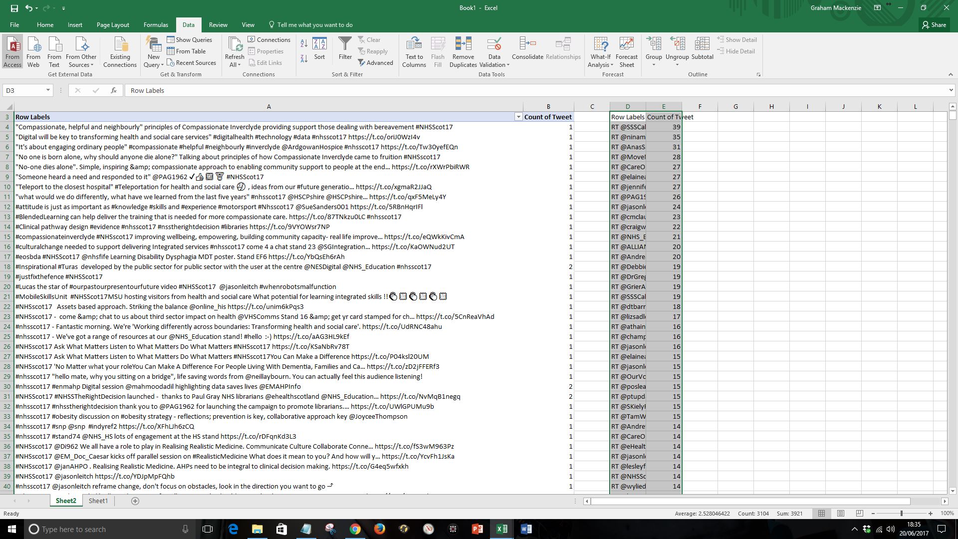
Step 12. The “Row Labels” column contains the texts of the different tweets. Some of these tweets will include mentions of other users (@username). Each mention of a user is recorded as a new relationship by NodeXL. This will be multiplied up with replies and retweets. Read more here. You need to take account of the number of “mentions” when you’re estimating number of retweets and can do this by copying the following formula into the adjacent column: =(LEN(D4)-LEN(SUBSTITUTE(D4,“@”,“”)))/LEN(“@”) (you’ll probably have to type this out as browser does strange things to formatting of inverted commas; you may need to change the cell reference D4 depending on how you have set up your spreadsheet)
Step 13. Label your new column “Mentions”. Label the next column “Count/mentions” and add the following formula in the cell below: =E4/F4 Again you’ll probably have to type this out rather than copying and pasting, and may need to change the cell references (E4 and F4) depending on where you’ve pasted your data in the sheet
Step 14. Copy these two new cells down to the bottom of the sheet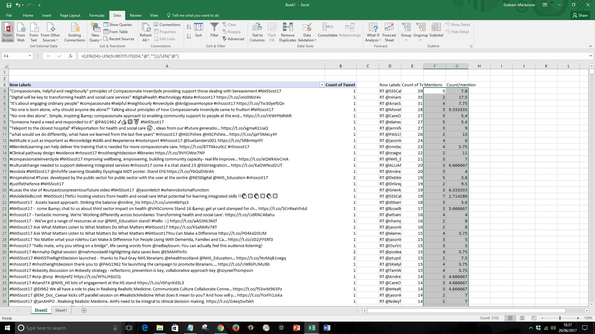
Step 15. Sort the columns by “count/ mentions” column (in decreasing order).
Step 16. Sort the columns by “count/ mentions” column (in decreasing order).
Step 17. Remove tweets with “#DIV/0” in “count/mentions” column. This might seem counter-intuitive, but these tweets will already be included in the analysis as retweets. Select the rows with the #DIV/0 tweets, and delete. Cut and paste the remaining rows just below the title row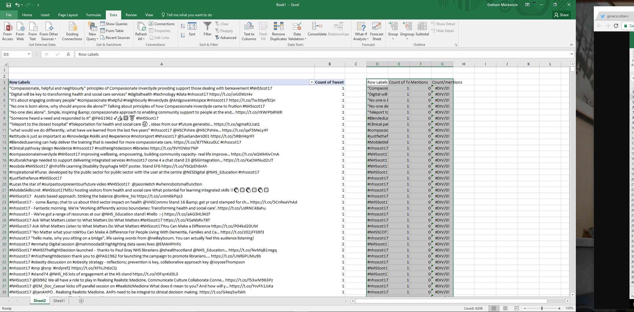
Step 18. Set up 3 new columns as shown, in preparation for recording URL, number of retweets (documenting when you recorded this information), and date and time of tweet (if you’re going to be ordering your tweets chronologically).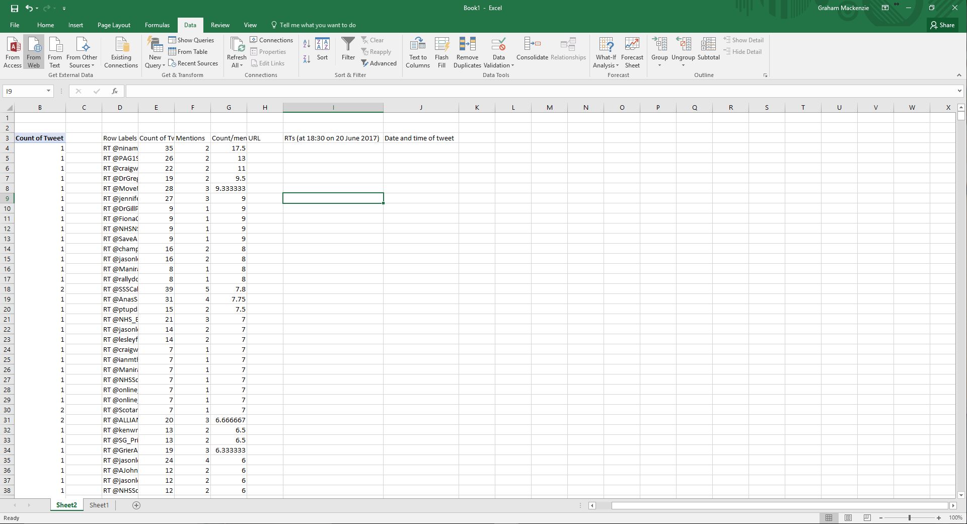
Step 19. Select a search term from the first tweet, avoiding URLs or hyphens at the start of the word (Twitter search uses hyphens as an instruction to exclude that term). You will need to identify which term work best for you using trial and error.
Step 20. Go to your browser. Enter the search term you’ve copied from Excel into the Twitter search box. Search through the different tweets if more than one appears and find the tweet that best matches sender and number of retweets. Once you’ve found the tweet click arrow in right hand side and click “Copy link to tweet”.
Step 21. Copy the link (control C).
Step 22. Paste the link into Excel (control V).
Step 23. Document the number of retweets identified from Twitter.
This step is only relevant if you’re going to order your tweets by time (eg for a conference). Step 24. Go back to browser and open up the tweet to extract the date and time it was posted (highlight by clicking on date, Control C to copy). Don’t worry if this is in a different time zone – it’ll be the same for all the tweets.
Step 25. Paste into Excel
Step 26. Repeat
Step 27. Order by number of retweets to identify the top tweets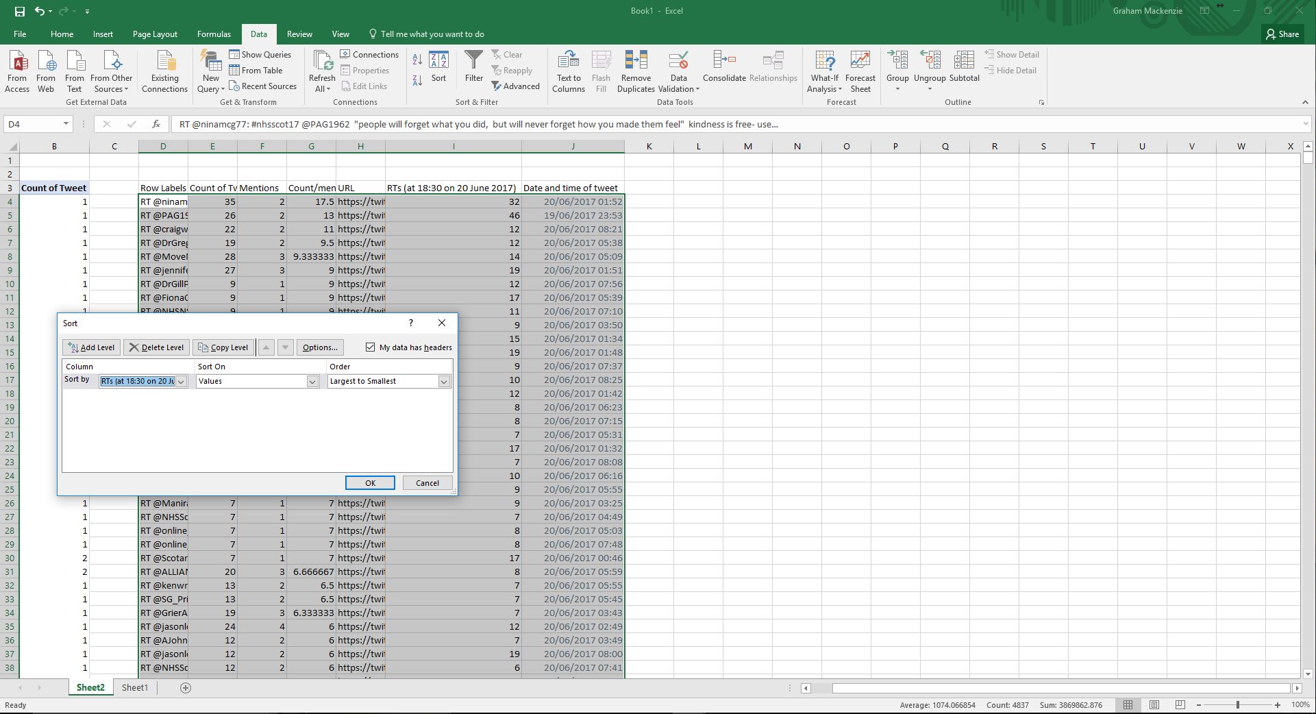
Step 28. Order chronologically if you are summarising a conference
Your data should look something like this depending on the rules you have applied – eg the number of retweets you are going to include, the weighting that you have given to different days etc
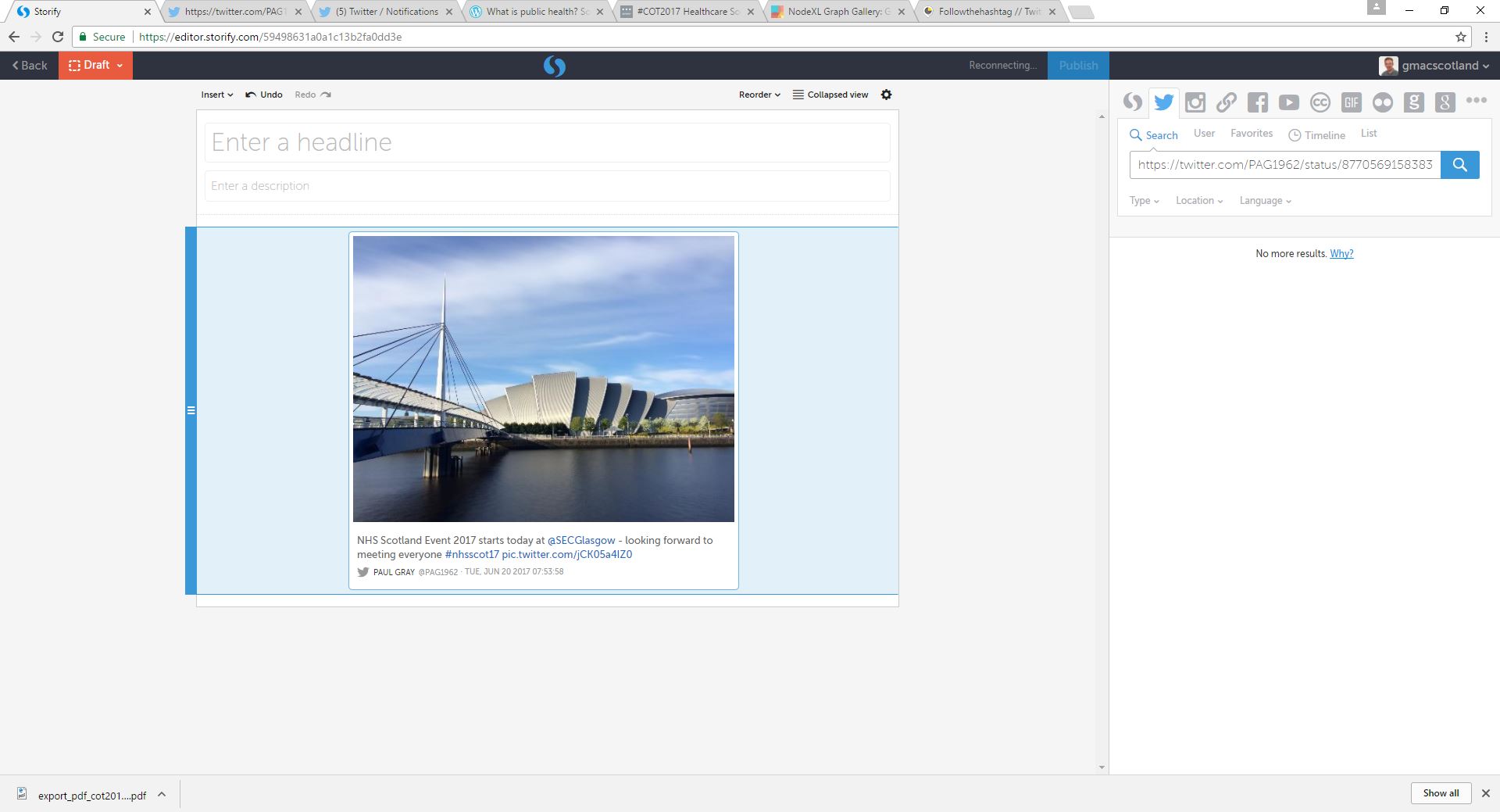
Step 29. You’re now going to use this information to produce a Storify summary. If you don’t have a Storify account set one up
Step 30. Find the individual tweets by taking the URLs in your Excel list and searching for them in Storify (click the Twitter logo, select search and paste the first URL)
Step 31. Storify will find the tweet
Step 32. Drag it across into the Storify summary – and repeat… Complete the title and description once you’re ready